Particle orientation refinement using GMM representation
- Most programs are available in EMAN2 builds after 2023-03, but some are still under continuous development. Newer versions are typically better.
- The tutorial is only tested on Linux with Nvidia GPU and CUDA.
For reference of the method, see the paper.
Here we use particles of SARS-COV-2 from EMPIAR-10492 as an example. Starting from particles with assigned orientation, i.e. the Polished folder (13.5GB) from EMPIAR, as well as job096_run_data.star.
Import existing refinement
Here we will need a .lst file with the location of all particles and their initial orientation assignment. Since here we start from a Relion star file, run
e2convertrelion.py job096_run_data.star --voltage 300 --cs 2.7 --apix 1.098 --amp 10 --skipheader 26 --onestack particles/particles_all.hdf --make3d --sym c3
Note that we need to phase flip the particles before the refinement, so this may take a while. Also make sure to provide the correct CTF related information to the program, including voltage, cs, amp, apix, since the program does not read those from the star file automatically. Check --help for more details. After importing the particles, with the --make3d option, the program will create a r3d_00 folder and reconstruct the 3D maps. You should see the structure of Covid spike with FSC at ~3.9Å at this point. Note the resolution number here is different from the one reported, because the pixel size used for processing is 1.098, which is then calibrated to 1.061. We still use the pixel size of 1.098 here, since otherwise the CTF information from the star file would be incorrect. Just keep in mind the actual resolution number is slightly better than the reported value.
To start from other formats:
From classical EMAN2 refinement (e2refine_easy), run e2evalrefine.py refine_XX --extractorientptcl particles.lst
From the new EMAN2 refinement (e2spa_refine), simply use the ptcls_XX.lst file from the last iteration.
From CryoSPARC or others, convert it to a relion star file using pyem, then follow the relion conversion.
To convert an EMAN2 lst back to the star file, use the --lst2star option. Note the two files need to be in the same order, so the even/odd lst files need to be merged and sorted first. For example, run
e2proclst.py gmm_00/ptcls_04_even.lst gmm_00/ptcls_04_odd.lst --create gmm_00/ptcls_04_all.lst --mergeref sets/all_relion.lst
to merge the particles while make sure the order is the same as the initial input, then run the same conversion command with the --lst2star option to generate a new star file.
e2convertrelion.py job096_run_data.star --voltage 300 --cs 2.7 --apix 1.098 --amp 10 --skipheader 26 --onestack particles/particles_all.hdf --lst2star sets/all_relion.lst
The new star file will be saved to job096_run_data_from_eman.star.
Global orientation refinement
To start the GMM-based refinement, we first need to determine the number of Gaussian to represent the volume. Often it is convenient to just use the number of non-H atoms in the molecule. Alternatively, we can guess the number given an existing map, isosurface threshold, and target resolution. Ideally, use a map with the correct masking, sharpening, and filtration, and pick an isosurface threshold where all features of interest are visible and most of the noisy dust is hidden. --maxres should be the target resolution, which can be slightly higher (0.4Å here) than the initially determined resolution. Having a slightly larger/smaller number normally does not hurt.
e2gmm_guess_n.py r3d_00/threed_00.hdf --thr 4 --maxres 3.5 --startn 10000
Here the number we get is 18000, and the program should also generate a file called r3d_00/threed_00_seg.pdb which can be used to visualize the coordinates of the Gaussian in the density map, and also used to initialize the GMM for refinement. The actual file name could be different depending on the e2gmm_guess_n command, and will be print out at the end of that command. Now we can run the GMM based global refinement.
e2gmm_refine_iter.py r3d_00/threed_00.hdf --startres 3.9 --initpts r3d_00/threed_00_seg.pdb --sym c3
The program will start from the initial orientation assignment and run five iterations of refinement using GMMs as references. It should create a folder called gmm_00, and you can find all files related to the refinement inside. threed_xx.hdf are the reconstructed density maps, fsc_masked_xx.txt are the FSC curves, and model_xx_even/odd.txt are the GMM parameters after each iteration. After the refinement, the resolution should reach ~3.4Å.
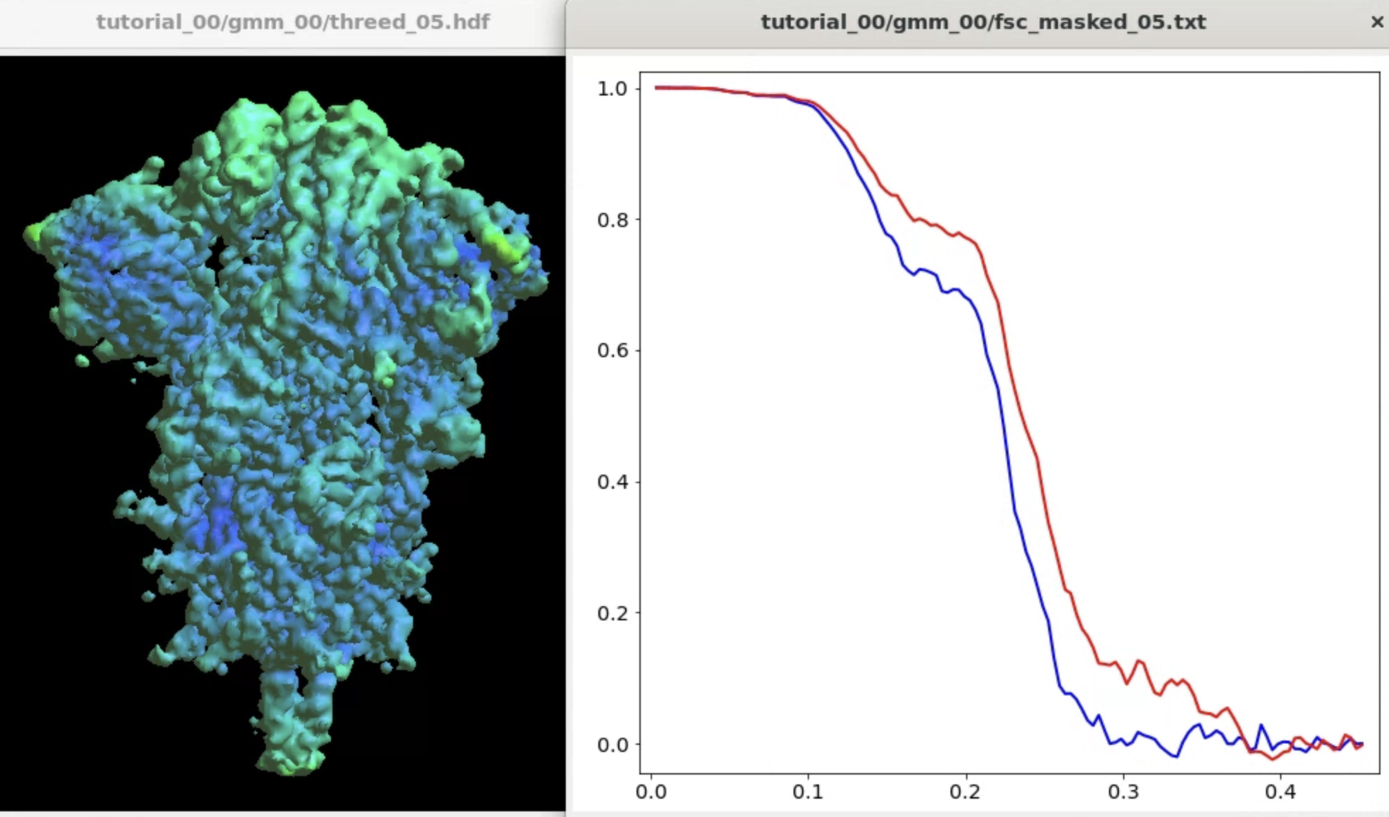
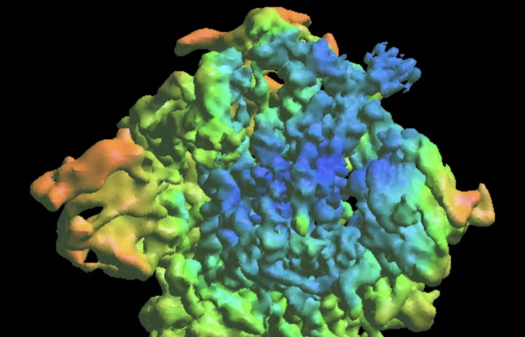
Note when displaying the volume through the Show3D button in e2display browser, the isosurface is automatically colored by the local resolution. Here we can see the tip of the spike is not as well-resolved as the central parts due to structual flexibility. We will address this in the following sections.
Focused refinement
Here we target the Receptor binding domain (RBD) using focused refinement. First, we need to make a mask for the target region using Filtertool. In the e2display browser, select gmm_00/threed_05.hdf and click Filtertool to start the program. Hold Shift while clicking the button will enter a "safe mode" of Filtertool, which might be useful if the program crashes often. To craft a mask for the RBD, we use three processors:
mask.soft:dx=15.0:dy=15.0:dz=80.0:outer_radius=20.0:width=20.0
filter.lowpass.gauss:cutoff_abs=0.2
mask.auto3d.thresh:nshells=4:nshellsgauss=6:return_mask=True:threshold1=6:threshold2=3.0
mask.soft locates the rough location of one of the RBD, and filter.lowpass.gauss lowpass filters the density map. mask.auto3d.thresh creates the final mask based on the filtered density. Basically, it starts from a high threshold indicated by threshold1, at which only the density of the target domain is visible, and gets down to a lower threshold2, where the density in the target domain is connected, but the density outside is not. The processor will then include all densities at threshold2 that are connected to the visible voxels at threshold1, pad a few layers and add a soft Gaussian falloff as indicated by nshells and nshellsgauss, then return the mask.
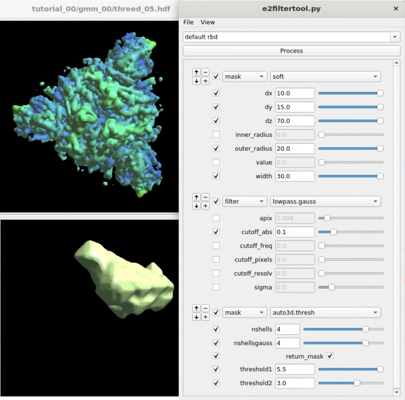
Clicking File -> Save will save the results to processed_map.hdf, and we rename it to mask_rbd.hdf for better bookkeeping.
Then run e2gmm_refine_iter.py again using the previous refinement and the new mask.
e2gmm_refine_iter.py gmm_00/threed_05.hdf --startres 3.5 --initpts gmm_00/model_04.txt --mask mask_rbd.hdf --masksigma --expandsym c3
Note here gmm_00/model_04.txt does not actually exist, but the program will look for gmm_00/model_04_even.txt and the odd version automatically, and keep the "gold-standard" split from the previous refinement. Since the global refinement is performed with c3 symmetry imposed, here we need to expand it to c1 to focus on one of the RBDs, i.e., making 3 copies of each particle at the symmetrical orientations.
The refinement will write related files in another gmm_xx folder. The final output will have a lower overall FSC curve, but better-resolved features at the target domain.
Refinement from a DNN heterogeneity analysis
For this dataset, we use the N terminal domain (NTD) as an example to show refinement starting from a heterogeneity analysis. The movement of NTD is actually relatively subtle, and there might not be a significant difference between DNN-based heterogeneity analysis and the focused alignment. Ideally, this function is more useful when the target domain involves large-scale (with a range of 10Å or more) continuous movement. Nonetheless, we use this as a demonstration since it is easier to show all functionalities in one small dataset.
Again, we start by making the mask for the NTD using the same method, and name the output mask_ntd.hdf
mask.soft:dx=30.0:dy=70.0:dz=70.0:outer_radius=20.0:width=30.0
filter.lowpass.gauss:cutoff_abs=0.1
mask.auto3d.thresh:nshells=4:nshellsgauss=4:return_mask=True:threshold1=3:threshold2=1
Then run the heterogeneous refinement starting from the previous global refinement given the mask for NTD.
e2gmm_heter_refine.py gmm_00/threed_05.hdf --mask mask_ntd.hdf --expandsym c3 --maxres 3.5 --minres 80
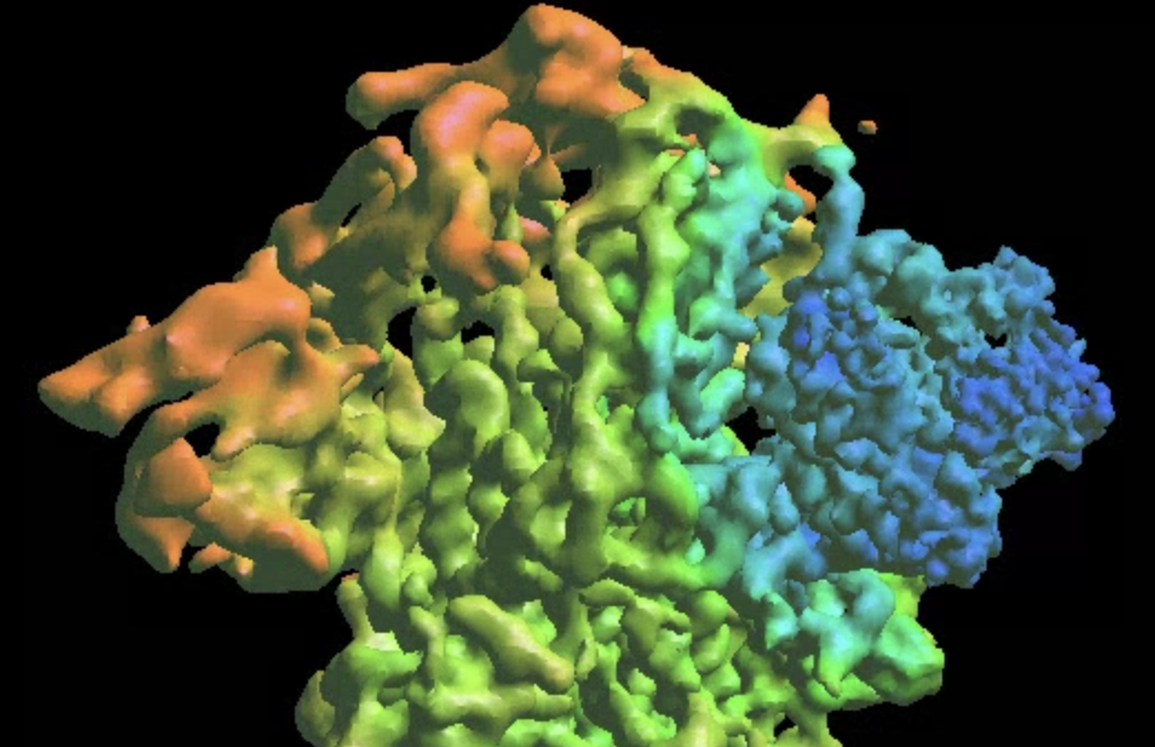
The program will first perform the DNN heterogeneity analysis on that domain, and the trajectories can be viewed in gmm_xx/ptcls_even_cls_00.hdf. Since we keep the "gold-standard" data separation through the pipeline, there will be one volume stack for each subset. The exact trajectory can be different but the overall movement pattern from the subsets should be similar.
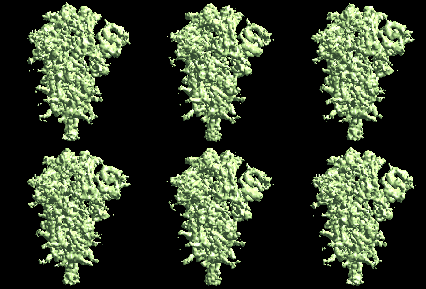
Then the program will convert conformation to particle orientation and perform a few rounds of focused alignment starting from the new orientation. This will produce a final map that is better resolved at one of the NTDs, and smeared out everywhere else.
Morphing molecular models
(Updated 2024-09) Now it is recommended to get the model series through the gmm_model protocol, which should generate models that match the heterogeneity analysis result and also have good geometry.
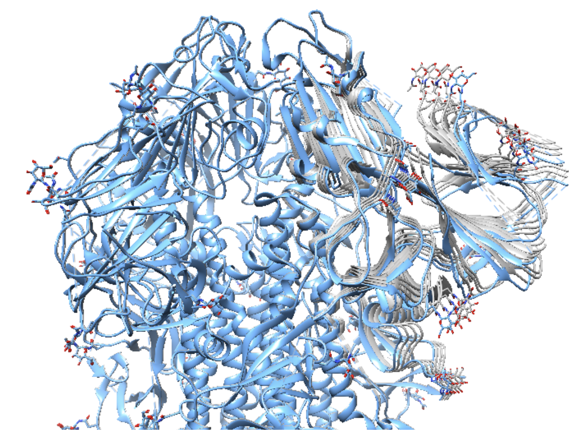
We can also visualize the same movement via molecular models. Here we use the existing PDB file (PDB:6zwv) and morph it using the trained decoder.
e2gmm_eval.py --pts gmm_04/midall_00_even.txt --pcaout gmm_04/mid_pca.txt --ptclsin gmm_04/ptcls_00_even.lst --ptclsout gmm_04/ptcls_even_cls_10.lst --mode regress --ncls 4 --nptcl 5000 --axis 0 --decoder gmm_04/dec_even.h5 --pdb 6zwv.pdb --apix 1.061 --selgauss mask_ntd.hdf --skip3d --model00 gmm_04/model_00_even.txt
Here gmm_04 was produced in the previous step of heterogeneity analysis with e2gmm_heter_refine. gmm_04/midall_00_even.txt is the latent space particle distribution of all particles from the even subset, focusing on the NTD, and gmm_04/dec_even.h5 is the corresponding trained decoder from the analysis. Due to the apix issue mentioned in the beginning, here we need to overwrite it using the --apix options so the model matches the density. The program should produce multiple pdb files corresponding to the individual frames of the 3D movie, which can be visualized in UCSF Chimera.
Merge multiple refinements
We also provide a simple way to merge the results from multiple refinement runs. For example, run
e2gmm_merge_patch.py gmm_01 gmm_02 --base gmm_00 --sym c3
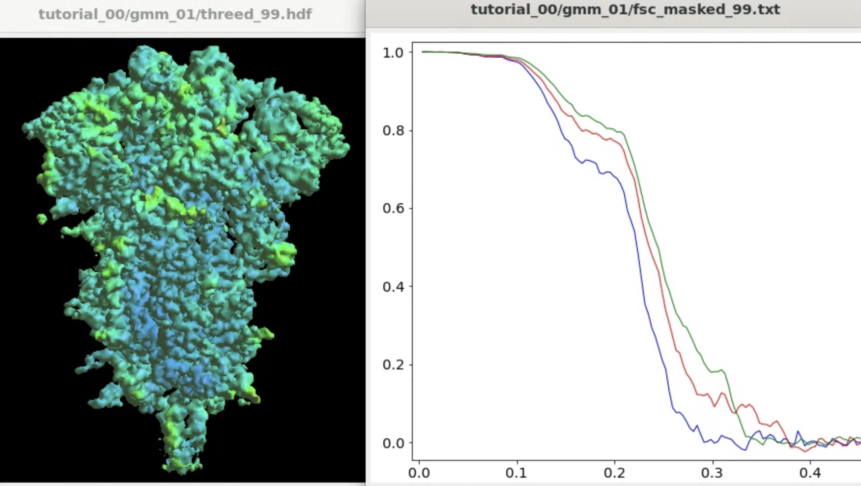
if you have the RBD and NTD refinement results in the gmm_01 and gmm_02 folders. It will take the results from gmm_00 as the base and replace the regions of focus using results from gmm_01 and gmm_02 and their corresponding focusing mask files. The program will use unmasked maps for the merge and recompute the FSC to filter the results accordingly. The result will be written as iteration 99 in the base folder, gmm_00.
Patch-by-patch refinement
Finally, we show the patch-by-patch refinement. This process is slow but automatic. In fact, since the scale of movement is relatively small in this particular dataset, the patch-by-patch refinement can render the steps after the global refinement quite useless. I.e., you can simply run this after the global orientation refinement, and get about as good or better results without the manual mask crafting and heterogeneity analysis. However, it is still worth trying the DNN-based analysis if the protein is undergoing large-scale continuous movement, or some domains are not as well resolved after the patch-by-patch refinement.
Starting from the global refinement, run
e2gmm_refine_patch.py gmm_00/threed_05.hdf --npatch 9 --startres 3.5 --masktight --expandsym c3
The program will divide the GMM into 9 patches and focus refine them individually. This will take 9 times longer than the focused refinement of one domain. The results of the patches will be merged together at the end and the final results will be shown as iteration 99.
Building motion trajectories from refinements
(After 2023-06-15) From the result of patch-by-patch refinement, or in fact any two or more refinement runs from the tutorial, we can build eigen-motion trajectories based on the difference of alignment of the same particles. For example, to assemble all results from the even half set of the patch-by-patch refinement, run
e2spa_trajfromrefine.py gmm_05/ptcls_*3_even.lst --baseali gmm_05/ptcls_00_even.lst
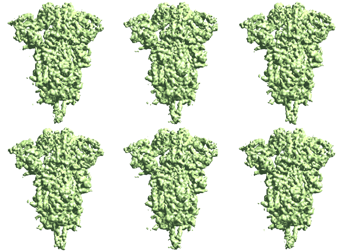
The movement is a bit subtle since we take information from all patches. You can also view trajectories from a selected local region by providing only the ptcls_xx.lst file focused on that region.
