Structural variability analysis with Gaussian mixture model (2022)

New (2022) version of the GMM based heterogeneity analysis workflow.

Significantly lower memory usage
Incorporate model information
Coordinated large-small scale movement

Example: EMPIAR-10059 particle stack

Note: some scripts are in the examples folder. It is recommended to add examples to PATH.

Start from converting relion particles to EMAN format. Make sure the particle path in the star file corresponds to the actual path. This will also perform CTF phase flipping per particle.

e2convertrelion.py particles.star --voltage 300 --cs 2 --amp 10 --apix 1.2156

Single model refinement. Here we skip the initial model generation and simply use the existing structure.This should get to ~3A within 10 iterations. To skip the refinement step, download the finished refinement folder here.

e2spa_refine.py --ptcl sets/all.lst --ref emd_8117.hdf --keep .9 --sym c4 --res 20 --parallel thread:32

Make a working folder for e2gmm, then copy the particle list and map file into it.

mkdir gmm_00
e2proc3d.py r3d_00/threed_13.hdf gmm_00/ref.hdf
e2proclst.py r3d_00/ptcls_13.lst --create gmm_00/ptcls_all.lst

Now make the neutral Gaussian model. First generate projections of the averaged map.

e2project3d.py gmm_00/ref.hdf --outfile gmm_00/projections.hdf --orientgen=eman:delta=5 --parallel=thread:12

Here we will seed the GMM from real space segmentation of the structure. With 8000 Gaussian functions, we can represent the structure at 3A resolution. If you have a model file of the protein in pdb, it is also possible to just use that to seed the GMM.

e2segment3d.py gmm_00/ref.hdf --pdb gmm_00/model_00.pdb --process=segment.kmeans:nseg=8000:thr=4

e2gmm_refine_new.py --ptclsin gmm_00/projections.hdf --model gmm_00/model_00.pdb --maxres 3. --modelout gmm_00/model_00.txt --niter 40 --trainmodel --evalmodel gmm_00/model_projs.hdf

Now look at the GMM in 3D. Use the same structure factor as the averaged map for better comparison. The map-model FSC should reach 3-4A.

e2proc3d.py gmm_00/ref.hdf gmm_00/ref.hdf --calcsf sf.txt

e2spa_make3d.py --input gmm_00/model_projs.hdf --output gmm_00/model_avg.hdf --threads 24 --setsf sf.txt

e2proc3d.py gmm_00/model_avg.hdf gmm_00/fsc_map_model.txt --calcfsc gmm_00/ref.hdf

In this tutorial, we only look at the domain outside the membrane, so we need to make a mask for it first. Here how sharp the map is actually does not matter. Alternatively, selecting atoms in Chimera and use a text file containing a list of Gaussian indices also works.

e2proc3d.py gmm_00/ref.hdf gmm_00/mask_sel.hdf --process=math.linear:scale=0:shift=1 --process=mask.zeroedge3d:z1=100 --process=filter.lowpass.gauss:cutoff_abs=0.1

Now prepare the particles for the heterogeneity analysis. The single model refinement was done with c4 symmetry applied, but the movement we are after may be asymmetric. To release the symmetry, run

cp gmm_00/ptcls_all.lst gmm_00/ptcls_all_sym.lst
e2proclst.py gmm_00/ptcls_all.lst --sym c4 --shuffle

Also we create a random subset for initial training to save time.

e2proclst.py gmm_00/ptcls_all.lst --create gmm_00/ptcls_sample.lst --range 50000

To look at large scale movement, we build a small model of only 32 anchor atoms.

e2segment3d.py gmm_00/ref.hdf --pdb gmm_00/model_01.pdb --process=segment.kmeans:nseg=32:thr=4
e2gmm_refine_new.py --ptclsin gmm_00/projections.hdf --model gmm_00/model_01.pdb --maxres 20 --modelout gmm_00/model_01.txt --niter 20 --trainmodel

Finally, everything is prepared, we can start the heterogeneity analysis. In the initial run, we target movement at the scale of 10A, using the anchor points.

e2gmm_refine_new.py --model gmm_00/model_00.txt --anchor gmm_00/model_01.txt --conv --midout gmm_00/mid_00.txt --maxres 10 --minres 40 --learnrate 1e-5 --niter 20 --ptclsin gmm_00/ptcls_sample.lst --heter --selgauss gmm_00/mask_sel.hdf --encoderout gmm_00/enc.h5 --decoderout gmm_00/dec.h5 --pas 100

We can also release the anchor points in a following run and target a higher resolution for the heterogeneity analysis. The step can be skipped.

e2gmm_refine_new.py --model gmm_00/model_00.txt --conv --midout gmm_00/mid_01.txt --maxres 10 --minres 40 --learnrate 1e-5 --niter 10 --ptclsin gmm_00/ptcls_sample.lst --heter --selgauss gmm_00/mask_sel.hdf --encoderin gmm_00/enc.h5 --decoderin gmm_00/dec.h5 --pas 100

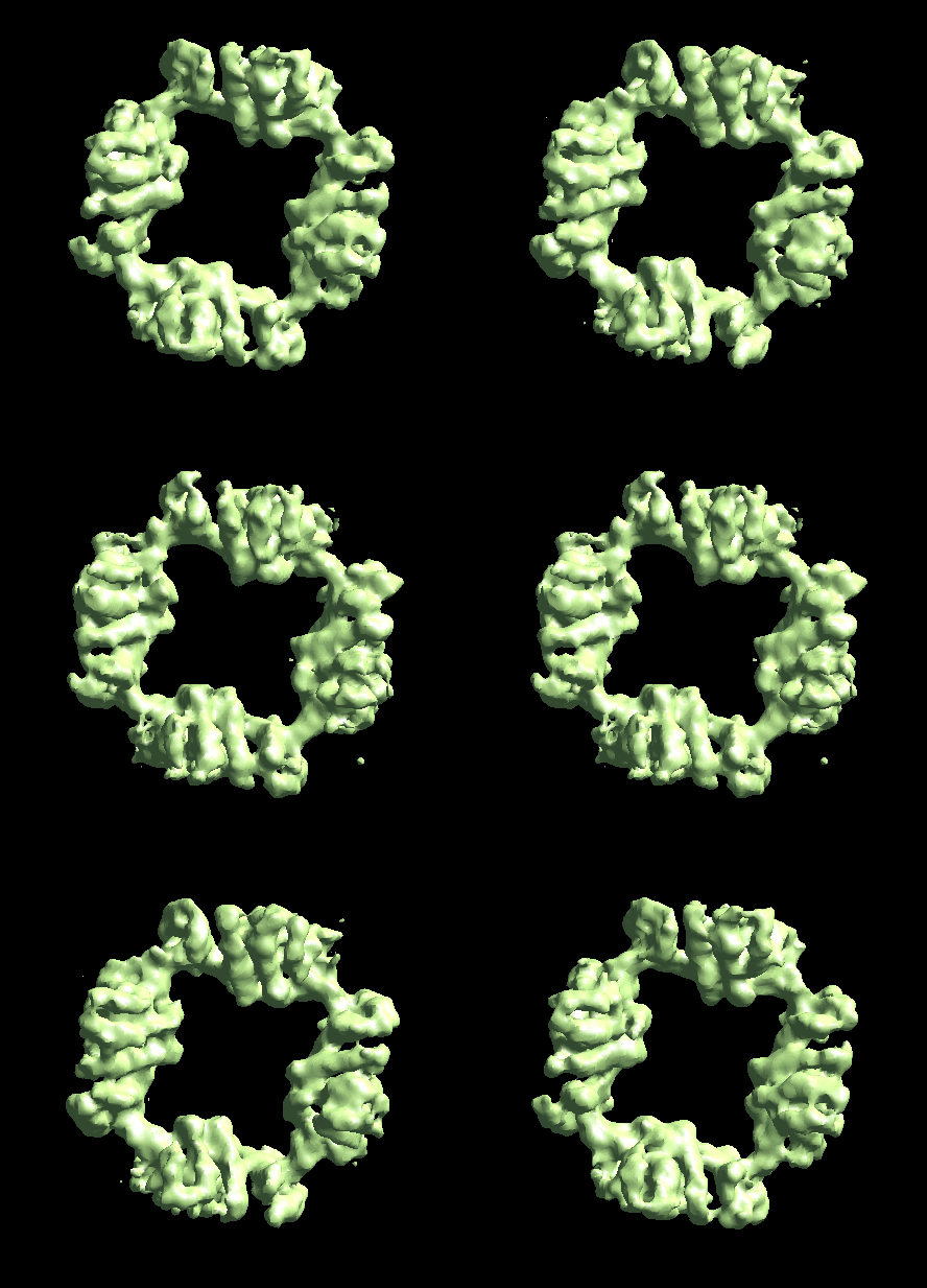
To look at the movement, we can reconstruct 3D maps along each eigen-axis of the conformation space.

ptcl_pca_kmean_m3d.py --pts gmm_00/mid.txt --pcaout gmm_00/mid_pca.txt --ptclsin gmm_00/ptcls_sample.lst --ptclsout gmm_00/ptcls_cls.lst --setsf sf_lp.txt --mode regress --ncls 5 --nptcl 8000 --axis 0

There are actually many degrees of freedom within the system, and it is a bit random which mode of motion will show up along the first axis. Explore and have fun...