|
Size: 17830
Comment:
|
Size: 17891
Comment:
|
| Deletions are marked like this. | Additions are marked like this. |
| Line 11: | Line 11: |
| First, make a new empty folder for the project, and run '''[[|e2projectmanager.py]]''' inside the folder. Make sure any command you run in the workflow are executed from this folder (not any subfolder inside). It is useful to change the project name and other properties from '''Project -> Edit project'''. They are not used by any program in the workflow, but it may help you keep track of things. Switch to the tomogram workflow tab using the menu next to Workflow mode. | First, make a new empty folder for the project, and run '''[[http://blake.bcm.edu/emanwiki/EMAN2/Programs/e2projectmanager|e2projectmanager.py]]''' inside the folder. Make sure any command you run in the workflow are executed from this folder (not any subfolder inside). It is useful to change the project name and other properties from '''Project -> Edit project'''. They are not used by any program in the workflow, but it may help you keep track of things. Switch to the tomogram workflow tab using the menu next to Workflow mode. |
EMAN2 Tomography Workflow Tutorial
This tutorial is suitable for EMAN2 source code after 09/27/2018. Most functionalities described in this tutorial are available in the 2.22 release.
Dataset
EMPIAR 10064 mixed CTEM, 4 tomograms.
Prepare input files
First, make a new empty folder for the project, and run e2projectmanager.py inside the folder. Make sure any command you run in the workflow are executed from this folder (not any subfolder inside). It is useful to change the project name and other properties from Project -> Edit project. They are not used by any program in the workflow, but it may help you keep track of things. Switch to the tomogram workflow tab using the menu next to Workflow mode.
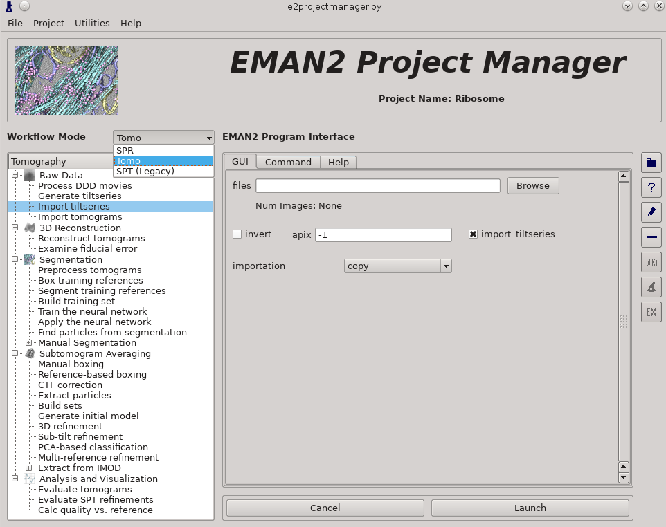
Import tilt series from your downloaded files using Raw Data -> Import tilt series. Select the files, and make sure importation says copy. Double check the Angstrom per pixel value of the tilt series (click info from e2display browser and look for apix_x). If it is not correct, specify the correct one in apix.
In the entire process, do not change the name of any files or move files between folders, since the program keep track of the metadata using file names. In general, files with the same base name, i.e. file name after the sub-folder name but before the double underscore (__), are considered coming from the same tomogram. The label/tag after the double underscore indicates the modification of the file. Their corresponding metadata, including alignment parameters, defocus, and particles can be viewed in the corresponding json file in the info directory.
Tomogram reconstruction
To first look at performance of the program, it is useful to start from one representative tilt series and turn off the notmp option, so temporary files will be written to tomorecon_XX. While default parameters works in most cases, slightly tweaking the parameters may produce more optimal results.
Make sure to set tltstep to be the angle between each tilt, in this case, 2 degrees. While the program can automatically compute the rotation of tilt axis, it is still better to fill in the correct value in tltax since there is a handedness ambiguity of the tomogram generated if the value is not provided.
In most cases, the default npk should work fine and it is not necessary to change the value according to the number of fiducial in images. When there are fewer (or no) fiducial in the tilt series, the program will use other high contrast object as landmarks.
Currently we only support output size of 1K and 2K which can be specified with the outsize option. In our experience, this is enough for visualization, annotation and particle picking. For subtomogram averaging, full sized particles will be generated from tilt series in the later steps.
In general, enabling bytile option can produce visually better result and make the program run faster. With this option, the program will generate tomogram in small tiles and merge them in real space. There are two things to keep in mind when using this option. First, the program will use multi-thread with this option and will consume more memory with a larger thread number. When there is not enough memory, especially when generating 2K output, the program might freeze the whole computer during reconstruction. Second, when there is large low resolution contrast in the tomogram, such as very thick cells, the edge between tiles may be visible, as there can be contrast difference between adjacent tiles.
When the sample is thin, it is useful to check correctrot to automatically position tomograms flat in ice. It also can be helpful to specify a clipz value to generate thinner tomograms.
When the sample is thick, consider check normslice, which can compensate the weaker contrast at the top and bottom of the tomogram.
After satisfied with the parameter selections, we can proceed to the whole dataset, simply check alltiltseries and uncheck notmp to reconstruct all tomograms sequentially.
Tomogram annotation
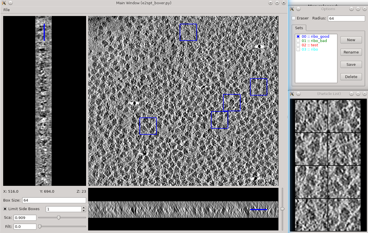
While it is unnecessary to automatically annotate the tomograms since the dataset we use for this tutorial are purified ribosomes, and can be easily picked by template matching, we still demonstrate the annotation process here to show how the annotation process connects to the following subtomogram averaging steps. A more detailed tutorial of the subject can be found in <link>. Note that some directory structure and user interfaces have changed in the latest version to keep with new tomogram workflow.
First preprocess the tomograms with the Preprocess tomograms command. This is not always necessary when the tomograms are reconstructed in EMAN2, but may still produce slightly better results. Next, box a few good and bad references in the Box training references step. We now switched to the new tomogram boxer GUI for particle picking which includes more functionalities. Go through slices along z axis using ‘~’ and ‘1’ on the keyboard.
You can now have different types of particles in the same tomogram, and add/rename/delete particle set in the set list window. Still it is better to keep the box size at 64 and shrink the tomogram for features of different sizes. As long as the tomograms are shrinked in EMAN, the boxer will keep track of the correct box sizes and coordinates in different versions of the same tomogram. In this case, we just need two classes of particles, ribo_good and ribo_bad. When clicking the Save button, all particles visible (with the box checked in front of the particle name) will be saved into one stack file. So in a more complicated cellular case, for example, one can have particles types of ribosome, microtubule, noise, and save (ribosome + noise) as negative training set for microtubules.
The rest of the annotation process remain unchanged, except for now all trained neural networks and training results are saved in the neuralnets folder, and all segmented maps are in the segmentations folder. You can now only specify the label of the output file instead of the full file name so the program can keep track of the metadata.
Finally, to turn segmented maps into particle coordinates, go to Find particles from segmentation, and input both the tomogram and its corresponding segmentation, and the particles coordinates will be written into the metadata file. Slightly tweaking the threshold parameters may yield better results. Here featurename will become the label of particles generated. Those particles can be viewed in the particle picking step and processed in the following protocols.
Particle picking
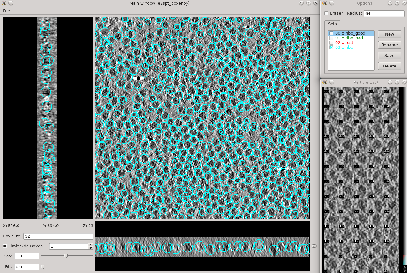
Launch the boxer in Subtomogram averaging -> Manual boxing step. You can also launch it via the Tomogram evaluation step which is discussed later in this tutorial. The interface is similar to the boxer used in the annotation step, except the boxes are shown as circles, whose radius indicates the distance from the current slice to the center of particle. Here we set the box size to be 45 for ribosomes. In this case, we can take a look at the automatically generated particles and remove some obvious bad ones. While you can save 3D particles from the GUI, there is no need to do so in this step. When you are satisfied with the result, simply close the window.
CTF correction
For this example, simple go to CTF correction, check alltiltseries and launch the program. For general applications, make sure the voltage and cs is correct for your microscope. The first two options, dfrange and psrange indicate the defocus and phase shift range to search. They take the format of “start,end,step”, so “2,5,.1” will search defocus from 2 to 5 um with a step size of 0.1. Unit for phase shift is degree. For defocused micrographs, we usually search a range slightly larger than the target defocus range. For images taken with volta phase plate, we usually have dfrange of “0.2,2,0.1” and psrange of “60,120,2”.
The program estimate the CTF taking the tilt angle of each image into consideration, so it only works after tomograms are reconstructed in EMAN. Note in this case, the program only determine the defocus of each tilt image, but does not correct for the CTF. CTF correction will be done at a per particle per tilt level in the next step.
Particle extraction
In this step, the program will extract unbinned 2D particles from tilt series, perform per particle per tilt CTF correction, then reconstruct individual 3D particles. Select Extract particles from the left panel, check alltomograms, and specify the label of particle you want to extract. Make sure the label specified here corresponds to the label of particles from the particle boxer. If the box size is correct when you select particles from the GUI, you can leave boxsz_unbin as -1, so the program will keep that box size. You can adjust the value if you want to change the box size of the extracted particles. With CTF information present, it generally does not hurt to check wiener, which filters the 2D particles by SSNR before reconstruct them into 3D. If you want to generate particles without CTF correction, check noctf. By default, the generated particles will have the same label as they are named in the boxer. If you want to have multiple types of particles, for example, with and without CTF correction, you can specify a different newlabel each time you launch the program.
Go to Build set in the left panel, check allparticles, and click launch. This will generate particle sets, which are virtual particle stacks that consist particles with the same label from different tomograms.
Initial model generation
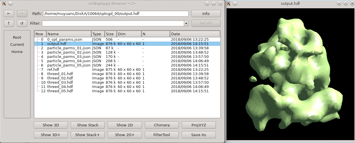
To build an initial model from scratch, simply go to the Generate initial model step and input the particle list. If you wish the process to be faster, set shrink to 2-4. It is not necessary to change other options. The program is parallelized, but not in a standard EMAN way. To use more cores, you can enter a bigger number in batchsize. This will not make the program run faster, but may make it converge to the correct answer faster. Also using more particles as input won’t make it run faster either, so just input the full particle set is fine. If the protein is known to be symmetrical, specify the correct symmetry. The program will not actually apply the symmetry (unless you check the applysym box, which is not recommended in general), but it will align the initial model to the symmetry axis so the following steps can work. For most situations, the default number of iterations (niter) of 5 is much more than needed. In this ribosome dataset with shrink 2, the program will converge to a good initial model before the end of the first iteration, usually within 10 minutes. Output files are written in folders called sptsgd_XX. In the output folder, the file output.hdf is the current initial model, which is updated after each batch (so 10-20 times per iteration). So it is okay to stop the program early and use the file as initial model once it looks good enough. While it would be good to have a better stopping criteria, given the diversity of things in cell, we have not come up with one yet.
Subtomogram refinement
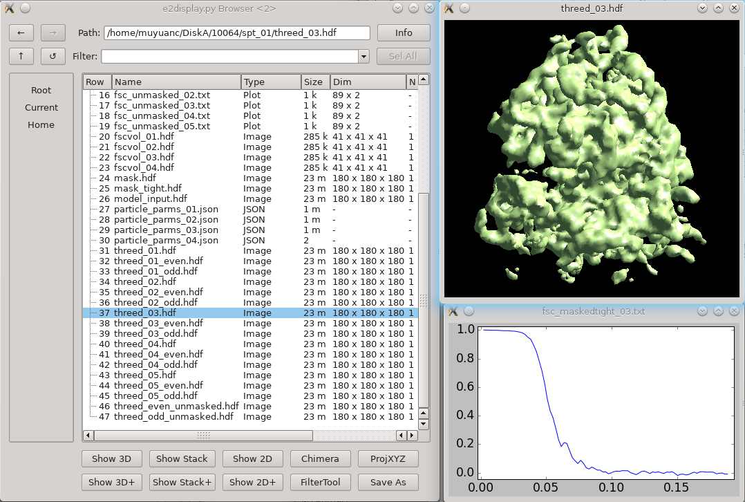
Click 3D refinement from the left panel, and input both the particle set and the initial model generated from the last step as reference. If there is a symmetry of the protein, make sure it is aligned to the symmetry axis before specifying the correct symmetry. If you are willing to split the even/odd set of particles and do a “gold-standard” refinement, specify a resolution number (usually 30-50) in goldstandard, so information beyond that resolution will be randomized independently in the reference for even and odd set. While it is good to have a reasonable mass for the molecular weight of protein (in kDa) and tarres for the target resolution, leaving them as default usually does not hurt. If you have a known structure factor in txt file, (you can compute it from a known structure via e2proc3d.py), specify it in setsf. localfilter will filter the averaged map by local resolution, which is especially useful when looking at things in cell where part of the protein can be very flexible. pkeep controls the fraction of particles that goes into the final average. If you know there are many bad particles in the dataset, setting it to be a smaller number may help. Enter the number of threads you want to use in the thread option. Finally, click Launch and wait. For this dataset, it can take a few hours on a descent workstation. The results can be seen in the spt_XX folder. In the folder, threed_XX.hdf are the main output map after each iteration, and fsc_masked/unmasked/masktight_XX.txt are the FSC curves between even/odd half set under different masking.
Subtilt refinement
Once the subtomogram refinement finishes, check the final map and FSC curves. In this dataset, it should get to 13-15A resolution. Now we can refine the orientation of each individual subtilt, i.e. 2D particles from raw tilt series that are reconstructed into to the 3D particles, and push the resolution of the averaged map. Click Sub-tilt refinement, choose the folder of the last subtomogram refinement and launch the program. The default parameters should be generally fine for this dataset. keep controls the fraction of particles that goes into the final map. If you are certain that tilt images beyond a certain angle (for example, 45 degrees) are radiation damaged, you can put 45 in maxalt, and specify a larger keep number. Otherwise, just use keep 0.5, so the program will judge the quality of subtilt images by their correlation to the averaged map and exclude worst 50% 2D particles.
Tomogram evaluation
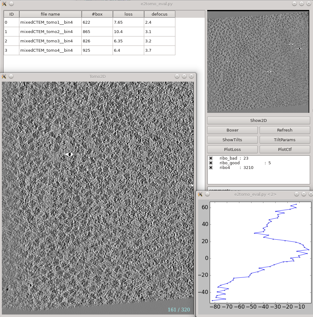
This is a tool that helps you visualize your tomograms with their corresponding metadata, and launch other programs from it. It can be found via Analysis and visualization -> Evaluate tomograms. This can be used at any point of the workflow after tomogram reconstruction.
On the left is a list of tomograms in the project. Clicking the header of each column will sort the table by that attribute. #box is the number of boxes in the tomogram, loss is the average fiducial error in nm, and defocus is the average defocus of the tilt series. Do not be scared by large loss values here. Although the relative value of different tomograms (aligned with the same parameters) in the same project is correlated to the quality of tilt series, the exact value here is not as meaningful. You can still get a subnanometer resolution subtomogram average from tilt series with a loss larger than 5 nm.
On the right, the image on the top shows the center slice of the tomogram. The Show2D button shows the selected tomogram in slices, ShowTilts shows the corresponding raw tilt series, and Boxer calls the 3D boxer. PlotLoss will plot the fiducial error per each tilt, and PlotCtf plot the defocus and phase shift at the center of image for each tilt. Tiltparams is a bit more complicated. It plots a point list with 6 columns and a number of rows corresponding to the images in the selected tilt series. These are the alignment parameters for the tilt series. The columns represent tilt ID, translation along x and y axis, tilt angle around y, x and z axis correspondingly. You can adjust X Col and Y Col in the plot control panel (middle click the plot) to change the display. The first panel below the buttons are the types of particle and their numbers in the dataset. Check and uncheck the boxes will affect the number displayed in #box column on the left. The last box is reserved for comments for each tomogram. You can fill in any comments you have for the selected tomogram and it will be saved with other metadata of the tomogram for future references.
Refinement evaluation
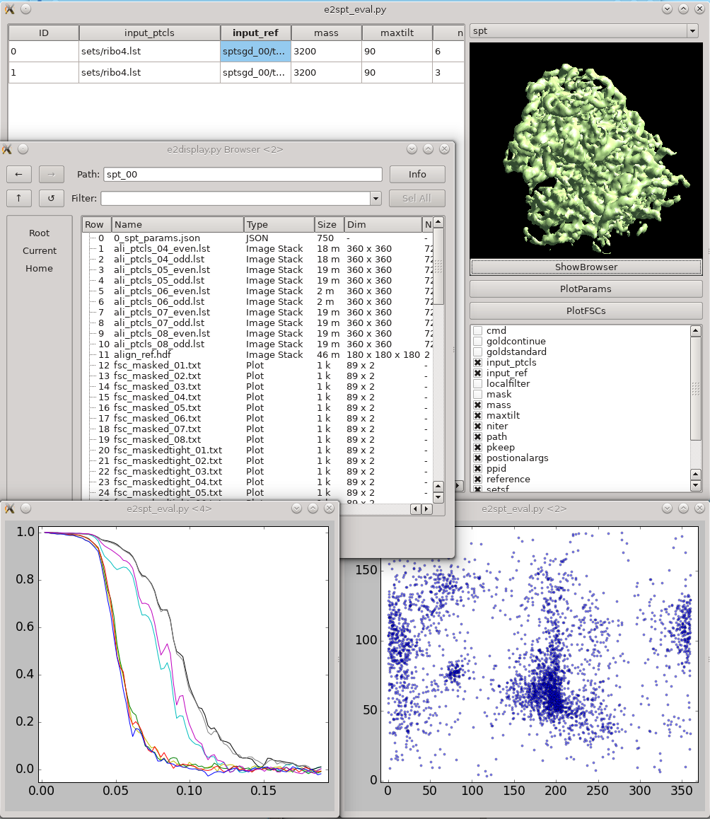
This tool helps visualize and compare results from multiple subtomogram refinement runs. Launch it from Analysis and visualization -> Evaluate SPT refinement. In the GUI, you can look at all spt_XX and sptsgd_XX folders and compare their options and resulting maps. Switch between type of folders using the menu at top right. Click the header of a column to sort the table by its content. Uncheck items in the list at bottom-right to hide corresponding columns. Clicking ShowBrowser will bring up the e2display.py browser in the folder of the selected row. PlotParams will plot the euler angle distribution and other alignment parameters.The 8 columns in the plot are three euler angles (az, alt, phi), translation in x,y,z, alignment score and missing wedge coverage score. PlotFSCs will plot the FSC curve under tight mask from each iteration.
