Structural variability analysis with Gaussian mixture model
Available in EMAN release after 10/01/2020. Still under development.
Dataset
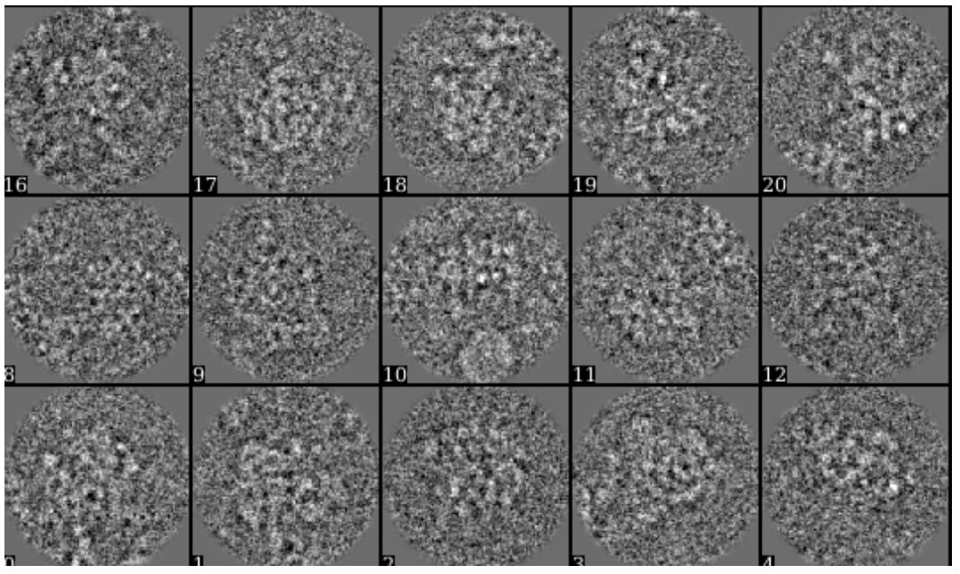
First, for the compositional heterogeneity analysis, we use the dataset of L17-Depleted 50S Ribosomal Intermediates from EMPIAR-10076. In this tutorial, we use a subset of only 6000 particles of box size 128. The particles are artificially selected to keep the tutorial is as simple as possible. To skip the alignment step, a single model refinement is run with the full dataset and the orientation of each particle is saved in the header of the image (xform.projection).
If you have previously run e2refine_easy on this data, you can extract the necessary files from a refine_XX folder using e2evalrefine.py with the --extractorientptcl option, and then just use the corresponding threed_XX file as a starting volume for the analysis.
The single model refinement can also be performed with the new e2spa_refine.py pipeline,which directly output the aligned list file and average density map that can be used as input.
To convert a refinement from Relion, a script called e2convertrelion.py can be found in the examples folder (after 01/2021) that produces phase flipped particles and aligned list file.
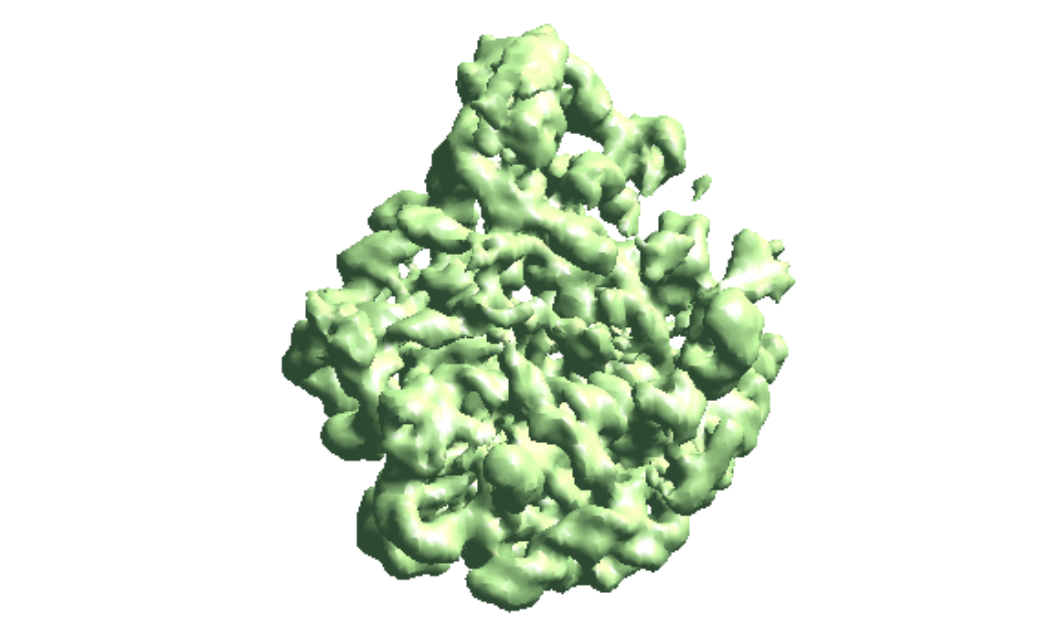
Reconstruct density map
Skip this step if you have an averaged map already. For the short tutorial, it is a useful step to double-check all the information in the particles is correct.
First, make the 3D map using the particles (or list file) with alignment information.
e2make3dpar.py --input ptcls_small.hdf --output avg.hdf --pad 192 --mode trilinear --keep 1 --threads 12
Now do a quick map sharpening for the output. The sharpened then filtered map is saved as avgsf.hdf. Also, create a structure factor file for the filtered map to simplify future reconstruction processes.
e2spt_structfac.py avg.hdf --res 15
e2proc3d.py avgsf.hdf avgsf.hdf --calcsf sf_lp.txt
Then make a mask and apply it to the map. The mask will be used to exclude Gaussian functions outside the boundary later. Now we have a “neutral” structure to start with.
e2proc3d.py avgsf.hdf msk.hdf --process=normalize.edgemean: --process=mask.auto3d.thresh:nshells=4:nshellsgauss=8:threshold1=5:threshold2=2:return_mask=1
e2proc3d.py avgsf.hdf avgmsk.hdf --process=normalize.edgemean --multfile msk.hdf
==Build the Gaussian model==
To limit memory consumption, the model is trained with 2D projections of the model instead of the 3D map. So here we make projections of the averaged map first.
e2project3d.py avgmsk.hdf --outfile avg_projs.hdf --orientgen=eman:delta=5 --parallel thread:12
Now we begin training the Gaussian model from scratch. We start from a tiny box size so it converges faster. Then run with a Fourier box size of 48 so the Gaussian model matches the density map at ~15 Å. The mask will exclude the Gaussian centers outside the volume. The second command can be repeated if the Gaussian model does not match well with the density map.
e2gmm_refine.py --projs avg_projs.hdf --npt 2048 --maxboxsz 24 --modelout model_gmm.txt --niter 20 --mask msk.hdf
e2gmm_refine.py --projs avg_projs.hdf --maxboxsz 48 --modelout model_gmm.txt --niter 20 --evalmodel model_projs.hdf --model model_gmm.txt --npt 2048  --mask msk.hdf
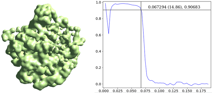
The --evalmodel option of e2gmm_refine.py will write the projection of the model to an image stack so we can take a look at the 3D reconstruction and check its FSC with the input density map.
e2make3dpar.py --input model_projs.hdf --output model_avg.hdf --pad 192 --mode trilinear --keep 1 --threads 12 --setsf sf_lp.txt
e2proc3d.py model_avg.hdf fsc_00.txt --calcfsc avgmsk.hdf
Heterogeneity analysis
Now we have a Gaussian model of the neutral structure, we can look into the heterogeneity of the particles. Run the e2gmm_refine.py command with particle input and --heter option to let the program embed them to a conformation space. The --gradout option writes the gradient with respect to the neutral structure to a file so the step can be skipped next time (read the saved file using --gradin). The middle layer output is saved in mid_00.txt. The --pas option controls the adjustment of position, amplitude, and sigma of the Gaussian functions. Setting it to 010 means changing amplitude only.
e2gmm_refine.py --model model_gmm.txt --ptclsin ptcls_small.hdf --heter --maxboxsz 48 --gradout allgrads.hdf --midout mid_00.txt --pas 010
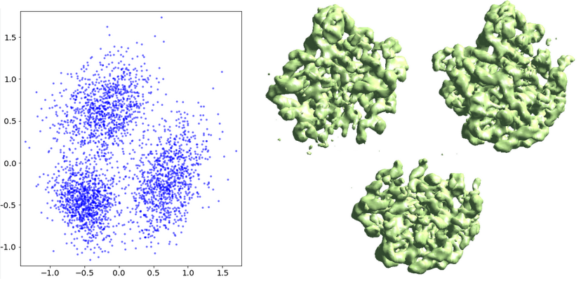
Finally, the ptcl_pca_kmean_m3d.py script (in examples folder) runs PCA on the middle layer output, classifies the particles, and reconstructs 3D maps of each class.
ptcl_pca_kmean_m3d.py --pts mid_00.txt --pcaout mid_pca.txt --ptclsin ptcls_small.hdf --ptclsout ptcls_cls --setsf sf_lp.txt


